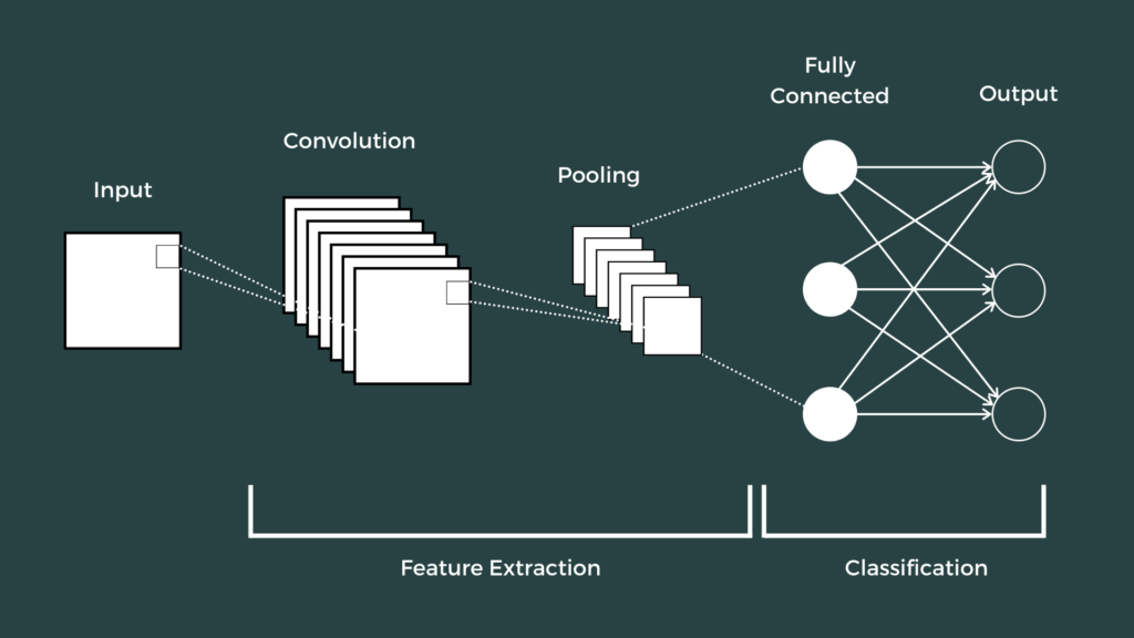
As we learned in the previous chapter, Neural Networks receive an input (a single vector), and transform it through a series of hidden layers. However, traditional neural networks do not perform well with images as the image vectors are usually very large.
For example, an image of size 224*224 when flattened is converted into a feature vector having 50,176 elements. As there will be 50,176 input nodes, and each input node should be connected to the node of another layer, the number of parameters in a network becomes quite large. This will make the network very large and inefficient. Hence, when working with images, we use a different type of neural network known as Convolutional Neural Networks (CNN). The following image shows the architecture of a Convolutional Neural Network,

If you want to have an even deeper understanding as to what Convolutional Neural Networks are, feel free to check this course.
In this chapter, we will be building a CNN to classify images of CIFAR10 dataset. The CIFAR10 dataset contains 60,000 color images in 10 classes, with 6,000 images in each class. The dataset is divided into 50,000 training images and 10,000 testing images. The classes are mutually exclusive and there is no overlap between them.
The CIFAR-10 dataset can be directly downloaded from the Tensorflow Dataset.
import tensorflow as tf

from tensorflow.keras import datasets, layers, models
import matplotlib.pyplot as plt

# Loading CIFAR-10 dataset
(train_images, train_labels), (test_images, test_labels) = datasets.cifar10.load_data()

# Normalize pixel values to be between 0 and 1
train_images, test_images = train_images / 255.0, test_images / 255.0
Downloading data from https://www.cs.toronto.edu/~kriz/cifar-10-python.tar.gz
170500096/170498071 [==============================] - 4s 0us/step
Let us have a better understanding of the dataset by visualizing some of the images in the dataset.
class_names = ['airplane', 'automobile', 'bird', 'cat', 'deer',
               'dog', 'frog', 'horse', 'ship', 'truck']

# Plot the images
plt.figure(figsize=(10,10))
for i in range(25):
    plt.subplot(5,5,i+1)
    plt.xticks([])
    plt.yticks([])
    plt.grid(False)
    plt.imshow(train_images[i], cmap=plt.cm.binary)
    plt.xlabel(class_names[train_labels[i][0]])
plt.show()

Now we define a convolutional network using a stack of Conv2D and MaxPooling2D layers.
As input, a CNN takes tensors of shape (image_height, image_width, color_channels). In this example, the CNN will take an input of shape (32, 32, 3), which is the format of CIFAR images.
# Initialize the model
model = models.Sequential()
model.add(layers.Conv2D(32, (3, 3), activation='relu', input_shape=(32, 32, 3)))
model.add(layers.MaxPooling2D((2, 2)))
model.add(layers.Conv2D(64, (3, 3), activation='relu'))
model.add(layers.MaxPooling2D((2, 2)))
model.add(layers.Conv2D(64, (3, 3), activation='relu'))

# Display the architecture
model.summary()
Model: "sequential_1"
_________________________________________________________________
Layer (type)                 Output Shape              Param #
=================================================================
conv2d (Conv2D)              (None, 30, 30, 32)        896
_________________________________________________________________
max_pooling2d (MaxPooling2D) (None, 15, 15, 32)        0
_________________________________________________________________
conv2d_1 (Conv2D)            (None, 13, 13, 64)        18496
_________________________________________________________________
max_pooling2d_1 (MaxPooling2 (None, 6, 6, 64)          0
_________________________________________________________________
conv2d_2 (Conv2D)            (None, 4, 4, 64)          36928
=================================================================
Total params: 56,320
Trainable params: 56,320
Non-trainable params: 0
_________________________________________________________________
After the convolutional layer, we will add a fully connected network (FCN) that will flatten the image from the maxpooling layer and perform classification.
model.add(layers.Flatten())
model.add(layers.Dense(64, activation='relu'))
model.add(layers.Dense(10))

# Display the architecture
model.summary()
Model: "sequential_1"
_________________________________________________________________
Layer (type)                 Output Shape              Param #
=================================================================
conv2d (Conv2D)              (None, 30, 30, 32)        896
_________________________________________________________________
max_pooling2d (MaxPooling2D) (None, 15, 15, 32)        0
_________________________________________________________________
conv2d_1 (Conv2D)            (None, 13, 13, 64)        18496
_________________________________________________________________
max_pooling2d_1 (MaxPooling2 (None, 6, 6, 64)          0
_________________________________________________________________
conv2d_2 (Conv2D)            (None, 4, 4, 64)          36928
_________________________________________________________________
flatten (Flatten)            (None, 1024)              0
_________________________________________________________________
dense (Dense)                (None, 64)                65600
_________________________________________________________________
dense_1 (Dense)              (None, 10)                650
=================================================================
Total params: 122,570
Trainable params: 122,570
Non-trainable params: 0
_________________________________________________________________
Finally, we compile our model using the adam optimizer. For loss function, we use the Sparse Categorical Cross Entropy. Then the model is trained for 10 epochs.
model.compile(optimizer='adam',
              loss=tf.keras.losses.SparseCategoricalCrossentropy(from_logits=True),
              metrics=['accuracy'])

history = model.fit(train_images, train_labels, epochs=10,
                    validation_data=(test_images, test_labels))
Epoch 1/10
1563/1563 [==============================] - 36s 23ms/step - loss: 1.5208 - accuracy: 0.4437 - val_loss: 1.2379 - val_accuracy: 0.5545
Epoch 2/10
1563/1563 [==============================] - 36s 23ms/step - loss: 1.1527 - accuracy: 0.5926 - val_loss: 1.1090 - val_accuracy: 0.6060
Epoch 3/10
1563/1563 [==============================] - 36s 23ms/step - loss: 1.0073 - accuracy: 0.6465 - val_loss: 0.9910 - val_accuracy: 0.6504
Epoch 4/10
1563/1563 [==============================] - 36s 23ms/step - loss: 0.9108 - accuracy: 0.6783 - val_loss: 0.9493 - val_accuracy: 0.6702
Epoch 5/10
1563/1563 [==============================] - 36s 23ms/step - loss: 0.8379 - accuracy: 0.7051 - val_loss: 0.9424 - val_accuracy: 0.6746
Epoch 6/10
1563/1563 [==============================] - 36s 23ms/step - loss: 0.7775 - accuracy: 0.7267 - val_loss: 0.8762 - val_accuracy: 0.7001
Epoch 7/10
1563/1563 [==============================] - 37s 23ms/step - loss: 0.7227 - accuracy: 0.7470 - val_loss: 0.8888 - val_accuracy: 0.6974
Epoch 8/10
1563/1563 [==============================] - 36s 23ms/step - loss: 0.6874 - accuracy: 0.7568 - val_loss: 0.9108 - val_accuracy: 0.6937
Epoch 9/10
1563/1563 [==============================] - 36s 23ms/step - loss: 0.6444 - accuracy: 0.7718 - val_loss: 0.9362 - val_accuracy: 0.6946
Epoch 10/10
1563/1563 [==============================] - 37s 24ms/step - loss: 0.6084 - accuracy: 0.7855 - val_loss: 0.8981 - val_accuracy: 0.7034
We now plot the training accuracy and validation accuracy to get a better insight of how well the model is trained.
# Visualizing the accuracy
plt.plot(history.history['accuracy'], label='accuracy')
plt.plot(history.history['val_accuracy'], label = 'val_accuracy')
plt.xlabel('Epoch')
plt.ylabel('Accuracy')
plt.ylim([0.5, 1])
plt.legend(loc='lower right')

test_loss, test_acc = model.evaluate(test_images,  test_labels, verbose=2)
313/313 - 3s - loss: 0.8981 - accuracy: 0.7034

From the above graph, we can see that as the training accuracy increases, the validation accuracy is decreasing. This might suggest overfitting. However, the methods for avoiding overfitting is out of the scope of this course. If you are interested, you can have a look at this article to get an idea of the methods you can use to avoid overfitting.
Do you want to learn Python, Data Science, and Machine Learning while getting certified? Here are some best selling Datacamp courses that we recommend you enroll in: